Analyzing Open Reading Frames of DNA Sequences using FASTA files
Master the skill of identifying and extracting open reading frames (ORFs). Delve into the fundamentals of biology, before embarking on a step-by-step journey through the ORF analysis process. You'll be able to grasp the algorithmic intricacies and gain a deeper understanding of the importance of ORF analysis.

DNA sequencing is a powerful tool that has transformed our understanding of genetics and biology by allowing us to determine the order of nucleotides in DNA. One of the many analyses that can be performed on nucleotide sequences is the identification of open reading frames, or ORFs for short. These regions of DNA or RNA sequences have the potential to be translated into protein sequences and can provide valuable insights into the biology of organisms.
In this article, we will explore the importance of ORFs, review the biological principles underlying their identification, and demonstrate how to analyze the ORFs of a DNA sequence stored in a FASTA file using Biopython, a popular and actively developed Python library for bioinformatics and computational biology. Additionally, we will introduce external tools for visualizing ORFs to help us better understand and interpret our results. By the end of this article, you'll have the knowledge and tools to search for and analyze ORFs in any DNA sequence of interest.
Central Dogma of Biology Basics
To understand how DNA's ORFs are analyzed, it's important to review the basics of the central dogma of biology. DNA, our genetic material, is made up of functional units called genes, which contain instructions for creating the proteins needed to perform functions in cells. That’s great, but how does a gene’s DNA sequence become a functional protein? This process involves two major steps: transcription and translation.
During transcription, a gene's DNA sequence is copied to create an RNA molecule. Since DNA is double-stranded and RNA is single-stranded, only one of the DNA strands is involved in transcription. Which one is used will affect the possible proteins that can be created. Lastly, in eukaryotes, RNA must undergo processing to become mRNA.
In translation, the sequence of mRNA is decoded into amino acids to create the protein. The mRNA nucleotides are read in groups of three called codons, with each codon corresponding to a specific amino acid. Some codons indicate where to start and stop translating for the protein.
This directional flow of information from DNA → RNA → protein during expression of a protein-coding gene is known as the central dogma of molecular biology. Understanding this process is essential for analyzing DNA's ORFs, which are sections of DNA that potentially code for proteins.
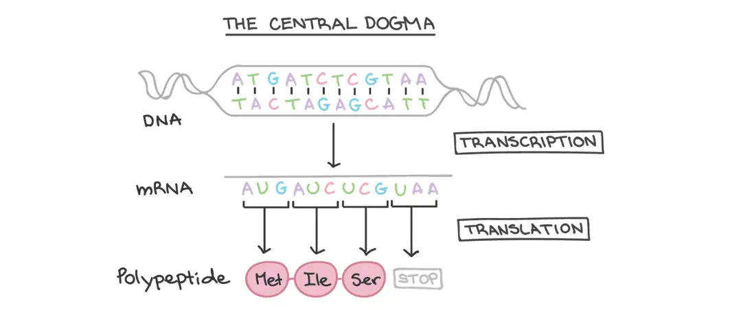
Picture from Khan Academy Intro to Gene Expression
Understanding the FASTA format
As previously mentioned, we will be reading DNA sequences from FASTA files. Let’s understand what these files are for and how they are structured.
What is a FASTA file?
A FASTA file is the most basic format for the storage of nucleotide and protein sequences. It is named after the FASTA software package, which was one of the first programs to use this format.
How are FASTA files structured?
A FASTA file consists of two main parts: a header and a sequence. The header starts with a greater than symbol (>) followed by a brief description or identifier of the sequence. This can include information such as the species or organism the sequence comes from, the gene name or ID, and other relevant details. The header line is followed by one or more lines containing the sequence data, which can be nucleotides or amino acids.
FASTA files can contain multiple sequences, each separated by a header line.
Here is an example of a simple FASTA file containing a short DNA sequence:
>seq1ATCGTAGCTAGCTAGCTGATCGTAGCTAGCTAGCTGATCGTAIn this example, >seq1 is the header, and the following line contains the DNA sequence.
Obtaining a sequence from a FASTA file
Let’s start by learning how to read and parse a sequence from a FASTA file using Biopython. Here is a simple example on how to do this:
from Bio import SeqIOfilename = "example.fasta"with open(filename, "r") as file: for seq_record in SeqIO.parse(file, "fasta"): print(seq_record.id) print(seq_record.seq)In this example, we want to read the sequences from the file example.fasta.
We first import the SeqIO module from Biopython, the standard Sequence Input/Output interface for BioPython, used to input and output assorted sequence file formats.
SeqIO.parse() is used to read in sequence data as SeqRecord objects. A SeqRecord is used in Biopython to hold a sequence with identifiers, description, and other optional annotations. SeqIO.parse() takes as arguments a (1) handle, previously created with the open() function, from which to read data from and a (2) lower case string specifying the sequence format. This function will return an iterator which gives SeqRecord objects for each sequence in the file.
Since we are returned an iterator, we must loop through the records to handle them one at a time. In this case, we use the id attribute of each SeqRecord object to print the identifier of the sequence, and the seq attribute to print the sequence data itself.
Analyzing the DNA sequence for ORFs
Importance of Open Reading Frames
Why might one want to analyze a sequence’s ORFs? Identifying ORFs is important in molecular biology for various reasons. I’ve included some of the points below:
- Gene annotation: ORFs can be used to identify genes in newly sequenced genomes by predicting the presence of protein-coding genes.
- Functional analysis: Predicted ORFs can provide insights into the function of proteins. By comparing the predicted protein sequences to known proteins, we can infer their potential function and contribute to our understanding of cellular processes.
- Drug target identification: ORFs can also be useful in drug discovery, where identifying proteins involved in disease pathways or critical to pathogen survival can lead to the development of targeted therapies.
Steps involved in identifying ORFs within a DNA sequence
So how do we actually extract all possible ORFs from a DNA sequence? Let’s go through the steps together:
Step 1: Read the DNA sequence
The first step in identifying ORFs is to obtain the DNA sequence from a database or file. In this example, we will extract the sequence from a FASTA file. It's important to ensure that the sequence is accurate and free from errors.
Step 2: Identify the reading frames
Let’s take a look at the following illustration to identify all the reading frames.
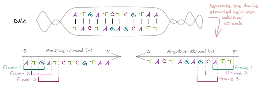
Since DNA is double stranded, we have two sequences of nucleotides from which RNA can be created. The individual DNA strands are called positive and negative strands, which must be read from 5’ to 3’. This leaves us with two strands that are reverse complementary of each other, meaning that which one is used as a template to generate the RNA will affect the possible ORFs we can find.
In addition, since the mRNA is read in triplets to translate to amino acids, depending on which position we start will affect the resulting amino acids. We can start reading from the 1st, 2nd, or 3rd nucleotide of the sequence, leaving us with three possible frames per sequence.
Therefore, to identify all possible ORFs, we need to analyze each of the six possible reading frames that result from combining the two strands and starting at three different positions.
To illustrate this, let's consider the six frames from the diagram:
| Frame | Positive Strand (+) | Negative Strand (-) |
|---|---|---|
| 5’ - ATGATCTCGTAA - 3' | 5’ - TTACGAGATCAT - 3’ | |
| 1 | ATG ATC TCG TAA | TTA CGA GAT CAT |
| 2 | A TGA TCT CGT AA | T TAC GAG ATC AT |
| 3 | AT GAT CTC GTA A | TT ACG AGA TCA T |
Once we have identified all possible reading frames, we can move on to the next step.
Step 3: Analyze each reading frame to extract the ORFs
Using the start codon "ATG" and stop codons "TAA," "TAG," or "TGA" in eukaryotic DNA, we can extract ORFs as subsequences of the DNA sequence that lie between a start and a stop codon. These sequences represent potential protein-coding regions within the DNA.
Step 4: Translate the ORFs
To determine the protein sequence, we need to translate the extracted ORFs into the corresponding amino acid using the genetic code. The genetic code is a set of rules that relate codons to specific amino acids.
Step 5: Analyze the ORFs
Finally, we can analyze the extracted ORFs to gain insights into gene function, structure, and evolution. We will not get to this step in this article, but I’ll expand upon these future analyses in the end.
Implementation of the algorithm
Since the ORFs need to be extracted from each frame independently, we will begin by creating a function that analyzes a single reading frame of a DNA sequence, returning a list of the ORFs found in said frame.
The code for this is as follows:
import mathCODON_SIZE = 3START_CODON = "ATG"END_CODONS = ["TAA", "TAG", "TGA"]def find_all_orfs_in_current_frame(seq, frame, strand, min_orf_len, max_orf_len): """ Finds all possible ORFs in the current reading frame by checking start and stop codons. Arguments: seq: the complete nucleotide sequence frame: the frame we are analyzing, either 0, 1 or 2 strand: identification of which DNA strand we are analyzing, positive (1) or negative (-1) min_orf_len: minimum length an ORF must have to be considered. max_orf_len: maximum length an ORF must have to be considered. Returns: list of subsequences of nucleotides between start and stop codons (ORFs). """ # Calculate where the reading frame starts and ends. Must be a multiple of 3. start = frame end = math.floor((len(seq) - frame)/CODON_SIZE) * CODON_SIZE + frame nucleotides = seq[start:end] # Where the ORFs sequences will be stored orfs_list = [] # Boolean indicating if a start codon was found => inside an ORF inside_orf = False # Loop through the sequence in steps of 3 (codon size) for i in range(0, len(nucleotides), CODON_SIZE): codon = str(nucleotides[i:i+CODON_SIZE]) # Start of an ORF if not inside_orf and codon == START_CODON: inside_orf = True orf_start_idx = i # End of an ORF elif inside_orf and codon in END_CODONS: inside_orf = False orf_end_idx = i + CODON_SIZE orf_len = orf_end_idx - orf_start_idx # Check if the ORF length is inside the limits if min_orf_len <= orf_len and orf_len <= max_orf_len: # Save the ORF to the list orfs_list.append(nucleotides[orf_start_idx:orf_end_idx]) return orfs_listSo what does the function find_all_orfs_in_current_frame do?
It starts off by establishing the start and end indexes we will be using given the frame, whose value can be 0, 1, or 2. Once we have the subsequence to use, we loop through this nucleotide sequence by codons. We store the current codon and analyze if it is a start or stop codon and if we are or are not inside an ORF.
If we have not have not previously found a start codon, and we fall upon one, we have found the start of an ORF. Hence, we store the current position as the start of the ORF and continue looping through the codons until we find a stop. Once this happens, if the length of the ORF is within the specified limits, we save the ORF in our array.
Now, we need a function that calls upon find_all_orfs_in_current_frame with the 6 possible reading frames. Let us view the code for this function.
from Bio import SeqIOdef analyze_orfs(fasta_input_file, min_orf_len, max_orf_len): # Open the input to create a handle with open(fasta_input_file, 'r') as input_file: # Parse all the sequences in the FASTA file and loop through each one for seq_record in SeqIO.parse(input_file, "fasta"): print('Working with Fasta sequence record %s' % seq_record.id) # To keep track of how many ORFs we have found => becomes the ORF's id orf_counter = 0 # Store the positive sequence = seq_record.seq # Store the negative strand => use Biopython's method that returns # the reverse complement of a sequence by creating a new Seq object reverse_sequence = sequence.reverse_complement() for strand, seq in [(1, sequence), (-1, reverse_sequence)]: for frame in range(0, 3): # Get the possible orfs of the frame frame_orfs = find_all_orfs_in_current_frame(seq, frame, strand, min_orf_len, max_orf_len) # Loop through all the ORFs for orf in frame_orfs: orf_counter += 1 # translate the nucleotide ORF sequence to amino acids protein_sequence = orf.translate(to_stop=True) print("ORF%i" % orf_counter) print(protein_sequence)The function analyze_orfs receives the filename of the FASTA file that contains the sequence and the limits to be placed upon the length of all ORFs. The function will retrieve the sequences from the FASTA files and convert them to SeqRecord as we learnt in the previous section, and for each record, extract, translate, and print all the ORFs in the six reading frames.
Let’s analyze more closely how to handle the six reading frames:
for strand, seq in [(1, sequence), (-1, reverse_sequence)]: for frame in range(0, 3): . . . These two for loops establish the six reading frames. We have two DNA strands we must analyze, the positive (1) and the negative (-1), and for each one, we must analyze the three reading frames.
# Get the possible orfs of the frameframe_orfs = find_all_orfs_in_current_frame(seq, frame, strand, min_orf_len, max_orf_len) for orf in frame_orfs: orf_counter += 1 # translate sequence to protein for a given ORF protein_sequence = orf.translate(to_stop=True) print("ORF%i" % orf_counter) print(protein_sequence)We then call upon our helper function, which returns all the ORFs in said frame. Each one of these ORFs must be translated into amino acids. For this, we use Biopython’s translation method, which turns a nucleotide sequence into a protein sequence by creating a new Seq object. The definition for this method is the following:
translate(self, table='Standard', stop_symbol='*', to_stop=False, cds=False, gap=None)
The arguments for this method are:
- table - Which codon table to use? We want the default Standard table since we need the standard genetic code table.
- stop_symbol - Stop codons will be translated to this single character string.
- to_stop - Boolean, indicates whether we want to continue the translation even if a stop codon is found. We do not want this, so we must set it as True.
- cds - Boolean, indicates this is a complete coding sequence. We do not want this check.
- gap - Single character string to denote symbol used for gaps. We will not worry about gaps for now.
To get a deeper understanding of this method, check out the official documentation here.
Lastly, we print to console the ORF’s id and the resulting amino acid sequence. However, it’s not very useful to simply print it to the console. Let’s move on to the next section to explore how to save the results to a new FASTA file.
Output and Visualization of ORFs
To improve our code, we can save the amino acid sequences of the identified ORFs in a FASTA file, along with additional information such as the start and end indexes of each ORF relative to the original sequence. This will enable us to compare our results with those of existing tools such as ORF Finder, which searches for ORFs in DNA sequences and provides a graphical representation of each ORF in its original sequence.
To gain a better understanding of how our program's output can be improved, we can examine an example and visualize the results of ORF Finder.
ORF Finder
Let’s take an mRNA sequence from NCBI, for example, a Homo Sapiens amylase sequence from this link. Now, let’s copy the sequence to ORF Finder, and leave the default parameters, which are:
- Minimal ORF Length (nt) = 75
- Want no ORFs smaller than 75 nucleotides.
- Genetic code = Standard
- Utilizing the standard genetic code table for translation.
- ORF start codon to use = “ATG” only
- Want to use only the eukaryotic start codon.
- Ignore nested ORFs = False
- Want to consider all possible ORFs, so do not ignore any.
This will result in the following visualization and information.
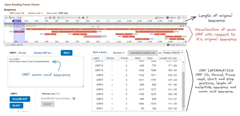
We can see that besides a graphical representation of the ORF, we have for each ORF the following information:
- Amino acid sequence
- Identification (counter)
- Which strand was used (+ or -)
- Which frame was used (1, 2, or 3)
- The start and end positions. Note how the negative strand’s ORFs have larger start positions than end positions. This is because the negative strand is analyzed in reverse order and the positions are relative to the original sequence.
- Length of the nucleotide and amino acid sequence
Let’s add this information to our output to improve our program's results and enable comparison with other existing tools.
Output improvement
First step to outputting more information is to save the information when extracting the ORFs. To do this, in the function find_all_orfs_in_current_frame, we make the following changes:
def find_all_orfs_in_current_frame(seq, frame, strand, min_orf_len, max_orf_len): # ... base_idx = 0 if strand == 1 else len(seq)-1 for i in range(0, len(nucleotides), CODON_SIZE): # ... elif inside_orf and codon in END_CODONS: # ... if min_orf_len <= orf_len and orf_len <= max_orf_len: orfs_list.append({ "seq": nucleotides[orf_start_idx:orf_end_idx], "start": base_idx + strand * (orf_start_idx + frame), "end": base_idx + strand * ((orf_end_idx - 1) + frame), "len": orf_len }) # ...This means we will now save the ORF sequence, its start and end position relative to the original sequence, and its length. Since orf_start_idx and orf_end_idx is relative to the frame we are analyzing, we must convert it to the indexes of the original sequence. We do this by adding the frame to our indexes and adding or subtracting it to the base_idx, depending on which strand we are on. The base_idx will represent the first index of each strand.
To save the results in a FASTA file, we must also make the following changes to analyze_orf:
#...from Bio.SeqRecord import SeqRecorddef analyze_orfs(fasta_input_file, output_file, min_orf_len, max_orf_len): orf_records = [] # Open the input and output to create the handles with open(fasta_input_file, 'r') as input_file, open(output_file, 'w') as orf_handle: for seq_record in SeqIO.parse(input_file, "fasta"): # ... for strand, seq in [(1, sequence), (-1, reverse_sequence)]: for frame in range(0, 3): # ... for orf in frame_orfs: # ... orf_records.append(SeqRecord( seq=protein_sequence, id= '%s_ORF%i' % (seq_record.id, orf_counter), description='|Frame %i|Strand %s|Pos[%i - %i]|Nt Len %i|AA Len %i|' % (frame + 1, ("+" if strand == 1 else "-"), orf["start"] + 1, orf["end"] + 1, orf["len"], len(protein_sequence)), )) # write to file SeqIO.write(orf_records, orf_handle, 'fasta')Each ORF is converted to a SeqRecord object and is saved in a list orf_records. The ID of the record will be the current record’s id followed by the ORF identifier. The description of this record will include all the information we established in the previous section.
Finally, we use SeqIO.write() to write the SeqRecords to the specified file. We pass to SeqIO.write() our list of records, our output file handler, and what type of file format we want to use. This function will automatically format the FASTA file with the headers and sequences. By adding this function outside the loop, we are writing to the file once and not one record at a time, hence, we are greatly improving our performance.
The resulting FASTA file will have the following format, which are easily comparable to those of ORF Finder:
>NM_001008221.1_ORF1 |Frame 2|Strand +|Pos[95 - 199]|Nt Len 105|AA Len 34|MSVFSTRGLVTSWLKTCLWKTSLAWNINSFWKGH...>NM_001008221.1_ORF13 |Frame 3|Strand -|Pos[948 - 778]|Nt Len 171|AA Len 56|MKGLLPSGNQLLFRLCSLSKIAFMSPGHMCLEASILNPATPMSMRWFIYSAILERTAnd we’re done! You have successfully used Biopython and your skills to extract all ORFs from a DNA sequence.
Wrap up
To wrap up, the identification of open reading frames (ORFs) in DNA sequences is a crucial step in drug discovery, understanding the functional and structural properties of proteins, identifying genes, and more. By using Biopython, a powerful Python library for bioinformatics and computational biology, we have learned how to extract ORFs from a DNA sequence stored in a FASTA file and translate them into amino acid sequences. With the knowledge gained from exploring external tools for visualizing ORFs, we have established important information to store when extracting ORFs.
With this knowledge and these tools at our disposal, we can continue to unravel the mysteries of the genetic code and gain a deeper understanding of the complex processes underlying life as we know it. We can continue our journey with the resulting ORFs by running BLAST consults to examine similar proteins across species, analyzing the protein’s motifs and domains, or running multiple sequence alignments with similar sequences. The opportunities are endless.
To view the complete project from this article, check out my biopython-playground in Github.
Happy coding!